Dear Student , 📚📝✨

During this task, you will implement a classifier using the ANN Class developed previously.

Task Description

1. Objective: Use an ANN to classify the (Q) transistor's state from the TCLab kit.

2. Research: Dive deep into the theory behind the ANN as classifiers. Again, I'd like you to explore textbooks, online resources, and real-world examples to understand how these methods work and when to use them.

3. Data collection:

   • Ensure your TCLab is working properly
   • Install the necessary Python libraries if you haven't already
   • You can use the following code to collect and tag your instances; we already did so in the previous lab session.
   • Do not forget to replace the aaa:bbb for the desired initial (aaa) and final (bbb) index to set ON the Q1
   • You must consider giving the transistor (Q1) enough time to reach the final temperature during the ON state and the OFF state.

    # 10 minute data collection
    import tclab, time
    import numpy as np
    import pandas as pd
    with tclab.TCLab() as lab:
    n = 600; on=100; t = np.linspace(0,n-1,n)
    Q1 = np.zeros(n); T1 = np.zeros(n) # to fill vectors with zeros
    Q1[20:41]=on; Q1[60:91]=on; Q1[150:181]=on.  # Adding the on state
    Q1[aaa:bbb]=on; Q1[aaa:bbb]=on; Q1[aaa:bbb]=on
    Q1[aaa:bbb]=on; Q1[aaa:bbb]=on; Q1[aaa:bbb]=on
    Q1[aaa:bbb]=on; Q1[aaa:bbb]=on; Q1[aaa:bbb]=on
    # Add more on states in the Q1 as you want
    print('Time Q1 T1')
    for i in range(n):
    T1[i] = lab.T1
    lab.Q1(Q1[i])
    if i%5==0:
    print(int(t[i]),Q1[i],T1[i])
    time.sleep(1)
    data = np.column_stack((t,Q1,T1))
    DF = pd.DataFrame(data,columns=['Time','Q1','T1'])
    DF.to_csv('data-classification.csv',index=False)
  

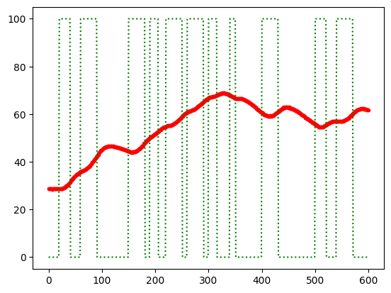
4. Explore your data: Before starting your classification task, use the next code to plot and visualize your data, and ensure your data is OK; avoid temperature data that is noisy or with slow changes (the plot from the beginning is a good-collected data):

    import matplotlib.pyplot as plt
    time = data[:,0]
    q = data[:,1]
    temp = data[:,2]
    plt.plot(time, temp,'.r')
    plt.plot(time, q, ':g')
    plt.show()
  

5. Load your data: Now load your data from the CSV file to split the data into training and test sets :

    import pandas as pd
    import numpy as np
    import matplotlib.pyplot as plt
    from sklearn.model_selection import train_test_split
    # Reading data from file:
    try:
    data = pd.read_csv('data-classification.csv')
    print('The data has been load and is stored in the `data` variable')
    except:
    print('Warning: Unable to load data-classification.csv, try to run first `data-collect.ipynb`')
  

6. Creating the additional features: Now compute the first and second derivatives, you can use numerical or approximations (you must research how to implement it) :

    # Input Features: Temperature, 1st and 2nd Derivatives
  
    # Add your propoussed code here ...
  

7. Scale the data and verify your targets: Scale the data if necessary and verify proper targets over instances.

8. Split the data: Remember to use separate or split data for the training and test data.

9. Implement your model and train it using your training sets (XA, YA)

    # Implement here your Supervised Classification
    from sklearn.linear_model import LogisticRegression
    # Your code here ...
  

10. Compare the model against your test data: Finally, you have to use the test data XB to compare your model against the real performance yB. Make a plot of the real Vs the model performance and show the best model to your professor; please include in the plot the temperature, first derivative, and second derivative on a proper scale.

11. Deadlines 📅: This session's deadline is the 25th of May.

12. Delivering the task 📄: This lab session does not require a report; add basic information to your Jupyter notebook file to explain to the professor what you did to make your classifier work.

13.  

Happy coding!

Gerardo Marx,

Lecturer of the Artificial Intelligence and Automation Course,

gerardo.cc@morelia.tecnm.mx